Mô tả:
1 Introduction
Field Precision finite-element programs covers a broad spectrum of physics and engineering
applications, including charged particle accelerators and X-ray imaging. The core underlying
most of our software packages is the calculation of electric and magnetic fields over three
dimensional volumes. To use our electric and magnetic fields software effectively, researchers
should have a background in electromagnetism and should be able to make informed decisions
about solution strategies. First-time users of finite-element software may feel intimidated by
these requirements. My motivation in writing this book is to share my experience in field
calculations. I hope to build users knowledge and experience in steps so they can apply finite
element programs confidently. In the end, readers will be able to solve real-world problems
with the following programs:
• EStat (2D electrostatics)
• HiPhi (3D electrostatics)
• PerMag (2D magnetostatics)
• Magnum (3D magnetostatics)
To begin, its important to recognize the difference between 2D and 3D programs. All finite
element programs solve fields in three-dimensions, but often systems have geometric symmetries
that can be utilized to reduce the amount of work. The term 2D applies to the following cases:
• Cylindrical systems with variations in r and z but no variation in θ (azimuth).
• Planar systems with variations in x and y and a long length in z.
Which brings us to the first directive of finite-element calculations: never use a 3D code for
a calculation that could be handled by a 2D code. The 3D calculation would increase the
complexity and run time with no payback in accuracy.
We need to clarify the meaning of static in electrostatics and magnetostatics. The implica
tion is that the fields are constant or vary slowly in time. The criterion of a slow variation is
that the systems do not emit electromagnetic radiation. Examples of electrostatic applications
are power lines, insulator design, paint coating, ink-jet printing and biological sorting. Magne
tostatic applications include MRI magnets, particle separation and permanent magnet devices.
A following coarse will cover simulations of electromagnetic radiation (e.g., microwave devices).
Secondly, its important to have a clear understanding of the purpose of computer calcula
tions of electric and magnetic fields. Numerical methods should be used when it is not possible
to generate accurate results with analytic methods. Numerical solutions are necessary in the
following circumstances: • The system has a complex asymmetric geometry.
• The solution volume contains many objects with different material properties.
• Materials have complex properties (e.g., saturation of iron in magnetic circuits)
In an ideal case, a user makes analytic estimates of field values and then applies numerical
methods to improve the accuracy. The initial analysis gives an understanding of the physics
involved and the anticipated scales of quantities – essential information for effective solution
setups. The worst case is when a user treats a program as an omniscient black box. No matter
what software manufacturers may claim, using a field program without understanding fields is
at best a gamble. Sometimes you may get lucky, but most of the time considerable effort is
wasted generating meaningless results.
In summary, I would like to help you become an informed software user. I suggest you
start by downloading a free textbook that will help you brush up on electric and magnetic field
theory. The book also gives a detailed description of the FEM techniques I will discuss:
S. Humphries, Finite-element Methods for Electromagnetics (CRC Press, Boca Raton,
1997) (available for free download at http://www.fieldp.com/femethods.html).
The following chapter describes how to download and to set up field-solution software packages.
2 Installing 2D electric-field software
In this chapter, we’ll discuss how to install and to test trial or purchased software. As a specific
example, consider a trial of the Electrostatics Toolkit for two-dimensional electric fields. To
request a trial, contact us a
[email protected]. You will receive an E mail message that
includes information like the following:
Name: Ernest Lawrence
Organization: LBL
Software: Electrostatics Toolkit
Date: August 20, 2014
Registration code: LAWRENCEER
Thanks for requesting a trial of Field Precision software. To download the
installer, please use this link:
Package: Electrostatics Toolkit Basic
Link: www.dsite.us/download/bin16/ElectrostaticsToolkitSetupBasic.exe
User: bin16
Password: BxHv7821%
Click the link to open it in your browser and copy-and-paste the User and Password infor
mation to start the download process. Save the file ElectrostaticsToolkitSetupBasic.exe
to a convenient location on your hard drive or a USB drive. If you have purchased the software,
be sure to keep a copy of the file in case you need to move the software or to install it on a
second computer.
When you run the installer, it sets up a directory containing programs, instruction manuals
and examples. A file manager is useful to check out the new materials. Because number
crunching finite-element programs produce a lot of data, a good file manager is a critical tool
for your future work. Figure 2 shows a screenshot of FP File Organizer, a free utility included
with our software.
If you check the root directory of the hard drive, youll see that the installer has created
the directory c:\fieldp basic (or c:\fieldp pro if you purchased the professional version).
Figure 2 shows the directory contents (left-hand side). The file readme basic.html is a useful
summary of instructions. The tricomp sub-directory (right-hand side) contains the programs,
documents and examples of the 2D package:
• dielectric constants.html. Relative dielectric constants for a variety of materials,
useful for setting up electrostatic solutions.
• estat.exe. The main solution program that combines information on the computational
mesh and material properties to find electrostatic potential values at nodes. The program
also creates graphs and plots of the solution (i.e., post-processing).
• estat.pdf. The EStat instruction manual. • estat conductive.cfg, estat dielectric.cfg and estat force.cfg. Configuration
files for the EStat post-processor for different types of electrostatic solutions.
• mesh.exe. The automatic mesh generator to create 2D conformal, triangular meshes.
• mesh.pdf. The instruction manual for Mesh.
• notify.exe and notify.wav. Utility programs to signal the completion of an automatic
batch run.
• PhysCons.pdf. A reference sheet of physical constants.
• tc.exe. An automatic controller for programs and resources of the 2D packages that we
will discuss in detail later.
The examples sub-directory contains directories of prepared examples for both the Mesh and
EStat programs (Figure 3). These examples can help you get off to a quick start. Well talk
about running them later. For now, well concentrate on getting all components running.
The Basic versions of our programs use Internet license management. The installer creates
a TriComp icon on your desktop (Fig. 4). Click on it to run tc.exe, the TriComp program
launcher. Well discuss the functions of the buttons latter. For now, click the Activation button
to launch FPSetup Basic.exe (Fig. 5, left-hand side). Click the License button, read the
license and then close the text window. Click the Setup button to open the activation dialog
(Fig. 5, right-hand side). Enter the registration code that we sent and pick any user name.
Check that you accept the terms of the license and click the Process button to receive a unique
Machine number for your computer. This number is copied to the clipboard.