Annals of Mathematics
The sharp quantitative
isoperimetric inequality
By N. Fusco, F. Maggi, and A. Pratelli
Annals of Mathematics, 168 (2008), 941–980
The sharp quantitative
isoperimetric inequality
By N. Fusco, F. Maggi, and A. Pratelli
Abstract
A quantitative sharp form of the classical isoperimetric inequality is proved,
thus giving a positive answer to a conjecture by Hall.
1. Introduction
The classical isoperimetric inequality states that if E is a Borel set in Rn ,
n ≥ 2, with finite Lebesgue measure |E|, then the ball with the same volume
has a lower perimeter, or, equivalently, that
(1.1)
nωn1/n |E|(n−1)/n ≤ P (E) .
Here P (E) denotes the distributional perimeter of E (which coincides with the
classical (n − 1)-dimensional measure of ∂E when E has a smooth boundary)
and ωn is the measure of the unit ball B in Rn . It is also well known that
equality holds in (1.1) if and only if E is a ball.
The history of the various proofs and different formulations of the isoperimetric inequality is definitely a very long and complex one. Therefore we shall
not even attempt to sketch it here, but we refer the reader to the many review
books and papers (e.g. [3], [18], [5], [21], [7], [13]) available on the subject
and to the original paper by De Giorgi [8] (see [9] for the English translation)
where (1.1) was proved for the first time in the general framework of sets of
finite perimeter.
In this paper we prove a quantitative version of the isoperimetric inequality. Inequalities of this kind have been named by Osserman [19] Bonnesen
type inequalities, following the results proved in the plane by Bonnesen in 1924
(see [4] and also [2]). More precisely, Osserman calls in this way any inequality
of the form
λ(E) ≤ P (E)2 − 4π|E| ,
valid for smooth sets E in the plane R2 , where the quantity λ(E) has the
following three properties: (i) λ(E) is nonnegative; (ii) λ(E) vanishes only
when E is a ball; (iii) λ(E) is a suitable measure of the “asymmetry” of E.
942
N. FUSCO, F. MAGGI, AND A. PRATELLI
In particular, any Bonnesen inequality implies the isoperimetric inequality as
well as the characterization of the equality case.
The study of Bonnesen type inequalities in higher dimension has been
carried on in recent times in [12], [16], [15]. In order to describe these results
let us introduce, for any Borel set E in Rn with 0 < |E| < ∞, the isoperimetric
deficit of E
D(E) :=
P (E)
1/n
nωn |E|(n−1)/n
−1=
P (E) − P (rB)
,
P (rB)
where r is the radius of the ball having the same volume as E, that is |E| =
rn |B|.
The paper [12] by Fuglede deals with convex sets. Namely, he proves that
if E is a convex set having the same volume of the unit ball B then
min{δH (E, x + B) : x ∈ Rn } ≤ C(n)D(E)α(n) ,
where δH (·, ·) denotes the Hausdorff distance between two sets and α(n) is a
suitable exponent depending on the dimension n. This result is sharp, in the
sense that in [12] examples are given showing that the exponent α(n) found in
the paper cannot be improved (at least if n 6= 3).
When dealing with general nonconvex sets, we cannot expect the isoperimetric deficit to control the Hausdorff distance from E to a ball. To see this it
is enough to take, in any dimension, the union of a large ball and a far away
tiny one or, if n ≥ 3, a connected set obtained by adding to a ball an arbitrarily
long (and suitably thin) “tentacle”. It is then clear that in this case a natural
notion of asymmetry is the so-called Fraenkel asymmetry of E, defined by
�
�
d(E, x + rB)
n
:
x
∈
R
,
λ(E) := min
rn
where r > 0 is again such that |E| = rn |B| and d(E, F ) = |E∆F | denotes the
measure of the symmetric difference between any two Borel sets E, F .
This kind of asymmetry has been considered by Hall, Hayman and Weitsman in [16] where it is proved that if E is a smooth open set with a sufficiently
small deficit D(E), then there exists a suitable straight line such that, denoting
by E ∗ the Steiner symmetral of E with respect to the line (see definition in
Section 3), one has
p
(1.2)
λ(E) ≤ C(n) λ(E ∗ ) .
Later on Hall proved in [15] that for any axially symmetric set F
p
(1.3)
λ(F ) ≤ C(n) D(F )
and thus, combining (1.3) (applied with F = E ∗ ) with (1.2), he was able to
conclude that
(1.4)
λ(E) ≤ C(n)D(E ∗ )1/4 ≤ C(n)D(E)1/4 ,
THE SHARP QUANTITATIVE ISOPERIMETRIC INEQUALITY
943
where the last inequality is immediate when one recalls that Steiner symmetrization lowers the perimeter, hence the deficit. Though both estimates (1.2)
and (1.3) are sharp, in the sense that one cannot replace the square root on the
right-hand side by any better power, the exponent 1/4 appearing in (1.4) does
not seem to be optimal. And in fact Hall himself conjectured that the term
D(E)1/4 should be replaced by the smaller term D(E)1/2 . If so, the resulting
inequality would be optimal, as one can easily check by taking an ellipsoid E
with n − 1 semiaxes of length 1 and the last one of length larger than 1.
We give a positive answer to Hall’s conjecture by proving the following
estimate.
Theorem 1.1. Let n ≥ 2. There exists a constant C(n) such that for
every Borel set E in Rn with 0 < |E| < ∞
p
(1.5)
λ(E) ≤ C(n) D(E) .
A few remarks are in order. As we have already observed, the exponent
1/2 in the above inequality is optimal and cannot be replaced by any bigger
power. Notice also that both λ(E) and D(E) are scale invariant; therefore it
is enough to prove (1.5) for sets of given measure. Thus, throughout the paper
we shall assume that
|E| = |B| .
Moreover, since λ(E) ≤ 2|B|, it is clear that one needs to prove Theorem 1.1
only for sets with a small isoperimetric deficit. In fact, if D(E) ≥ δ > 0, (1.5)
is trivially satisfied by taking a suitably large constant C(n). Finally, a more
or less standard truncation argument (see Lemma 5.1) shows that in order to
prove Theorem 1.1 it is enough to assume that E is contained in a suitably
large cube.
Let us now give a short description of how the proof goes. Apart from the
isoperimetric property of the sphere, we do not use any sophisticated technical
tool. On the contrary, the underlying idea is to reduce the problem, by means
of suitable geometric constructions, to the case of more and more symmetric
sets.
To be more precise, let us introduce the following definition, which will
play an important role in the sequel. We say that a Borel set E ⊆ Rn
is n-symmetric if E is symmetric with respect to n orthogonal hyperplanes
H1 , . . . , Hn . A simple, but important property of n-symmetric sets is that
the Fraenkel asymmetry λ(E) is equivalent to the distance from E to the ball
centered at the intersection x0 of the n hyperplanes Hi . In fact, we have (see
Lemma 2.2)
(1.6)
λ(E) ≤ d(E, x0 + B) ≤ 2n λ(E) .
944
N. FUSCO, F. MAGGI, AND A. PRATELLI
Coming back to the proof, the first step is to pass from a general set E to
a set E 0 symmetric with respect to a hyperplane, without losing too much in
terms of isoperimetric deficit and asymmetry, namely
(1.7)
λ(E) ≤ C(n)λ(E 0 )
and
D(E 0 ) ≤ C(n)D(E) .
A natural way to do this, could be to take any hyperplane dividing E in two
parts of equal measure and then to reflect one of them. In fact, calling E + and
E − the two resulting sets (see Figure 1.a), it is easily checked that
D(E + ) + D(E − ) ≤ 2D(E) ,
but, unfortunately, it is not true in general that
λ(E) ≤ C(n) max{λ(E + ), λ(E − )} .
E+
E+
E
E
E−
E−
(a) (b)
Figure 1: The sets E, E + and E −
This is clear if we take, for instance, E equal to the union of two slightly
shifted half-balls, as in Figure 1.b. However, if we take, instead, two orthogonal
hyperplanes, each one dividing E in two parts of equal volume, at least one of
the four sets thus obtained by reflection will satisfy (1.7) for a suitable constant
C(n) (see Lemma 2.5). Thus, iterating this procedure, we obtain a set with
(n − 1) symmetries and eventually, using a variant of this argument to get the
last symmetry, an n-symmetric set E 0 satisfying (1.7).
Once we have reduced the proof of Theorem 1.1 to the case of an
n-symmetric set E, equivalently to a set symmetric with respect to all coordinate
hyperplanes, all we have to do, thanks to (1.6), is to estimate d(E, B)
p
by D(E) (as x0 = 0).
To this aim we compare E with its Steiner symmetral E ∗ with respect to
one of the coordinate axes, say x1 . Simplifying a bit, the idea is to estimate
each one of the two terms appearing on the right-hand side of the triangular
inequality
(1.8)
d(E, B) ≤ d(E, E ∗ ) + d(E ∗ , B)
THE SHARP QUANTITATIVE ISOPERIMETRIC INEQUALITY
945
by the square root of the isoperimetric deficit. Concerning the first term, by
Fubini’s theorem we can write
Z
(1.9)
d(E, E ∗ ) =
H n−1 (Et ∆Et∗ ) dt ,
R
where, for any set F , Ft stands for {x ∈ F : x1 = t}. Since Et∗ is the
(n − 1)-dimensional ball with the same measure of Et , centered on the axis x1 ,
and since Et is symmetric with respect to the remaining (n − 1) coordinate
hyperplanes, by applying (1.6) –in one dimension less– to the set Et suitably
rescaled we get
(1.10)
H n−1 (Et ∆Et∗ ) ≤
2n−1 n−1
H
(Et )λn−1 (Et ) ≤ Cλn−1 (Et ) ,
ωn−1
where λn−1 (Et ) denotes the Fraenkel asymmetry of Et in Rn−1 . Then, assuming that Theorem 1.1 holds in dimension n − 1, we can estimate λn−1 (Et ) by
the deficit Dn−1 (Et ) of Et in Rn−1 , thus getting from (1.9) and (1.10)
Z
Z p
∗
d(E, E ) ≤ C
λn−1 (Et ) dt ≤ C
Dn−1 (Et ) dt .
R
R
Finally, by a suitable choice of the symmetrization axis xi , we are able to prove
that
Z p
p
Dn−1 (Et ) dt ≤ C D(E) ,
R
thus concluding from (1.6) and (1.8) that
p
p
λ(E) ≤ d(E, B) ≤ C D(E) + d(E ∗ , B) ≤ C D(E) + 2n λ(E ∗ ) .
p
∗ ) by
At this
point,
in
order
to
control
λ(E
D(E ∗ ), which in turn is smaller
p
than D(E), we could have relied on Hall’s inequality (1.3). However, we
have preferred to do otherwise. In fact in our case, since we may assume that
E is n-symmetric (and thus E ∗ is n-symmetric too) we can give a simpler, selfcontained proof, ultimately reducing the required estimate to the case of two
overlapping balls with the same radii (see the proof of Theorem 4.1). And this
particular case can be handled by elementary one-dimensional calculations.
The methods developed in this paper, besides giving a positive answer
to the question posed by Hall, can also be used to obtain an optimal quantitative version of the Sobolev inequality. This application is contained in the
forthcoming paper [14] by the same authors.
2. Reduction to n-symmetric sets
In this section, we aim to reduce ourselves to the case of a set with wide
symmetry, namely an n-symmetric one. Since, as will shall see in Section 5, we
may always reduce the proof of Theorem 1.1 to the case where E is contained
946
N. FUSCO, F. MAGGI, AND A. PRATELLI
in a suitably large cube Ql = (−l, l)n and |E| = |B|, we shall work here and in
the next two sections with uniformly bounded sets contained in
X := {E ⊆ Rn : E is Borel, |E| = |B|} .
And thus we shall use the convention that C = C(n, l) denotes a sufficiently
large constant, that may change from line to line, and that depends uniquely
on the dimension n and on l.
The whole section is devoted to show the following result.
Theorem 2.1. For every E ∈ X, E ⊆ Ql , there exists a set F ∈ X,
F ⊆ Q3l , symmetric with respect to n orthogonal hyperplanes and such that,
λ(E) ≤ C(n, l) λ(F ) ,
D(F ) ≤ 2n D(E) .
This section is divided into two subsections: in the first one, we collect
some technical properties needed later, and in the second we prove Theorem 2.1.
2.1. Some technical facts. In this subsection we collect some technical
facts to be used throughout the paper. Even though the ball centered in the
center of symmetry is in general not optimal for an n-symmetric set, the next
lemma states that this is true apart from a constant factor. In the sequel, for
any two sets E, F ⊆ Rn we shall denote by λ(E|F ) the Fraenkel asymmetry
relative to F , that is
�
�
d(E, x + rB)
λ(E|F ) := min
:
x
∈
F
,
rn
again being |E| = rn |B|.
Lemma 2.2. Let E ∈ X be a set symmetric with respect to k orthogonal
hyperplanes Hj = {x ∈ Rn : x · νj = 0} for 1 ≤ j ≤ k. Then one has
� � \k
�
λ E�
Hj ≤ 2k λ(E).
j=1
Proof. Let us set
�
Q− := x ∈ Rn : x · νj ≤ 0
�
Q+ := x ∈ Rn : x · νj ≥ 0
∀1 ≤ j ≤ k ,
∀1 ≤ j ≤ k .
By definition and by symmetry, λ(E) = d(E, p + B) for some point p ∈ Rn
belonging to Q− ; as an immediate consequence, denoting by p0 the orthogonal
T
projection of p on kj=1 Hj , one has that (p0 + B) ∩ Q+ ⊇ (p + B) ∩ Q+ . Hence,
�
�
E \ (p0 + B) ∩ Q+ ⊆ E \ (p + B) ∩ Q+ .
THE SHARP QUANTITATIVE ISOPERIMETRIC INEQUALITY
947
The conclusion follows just by noticing that, since both p0 + B and E are
symmetric with respect to the hyperplanes Hj ,
�
� \k
�
Hj ≤ d E, (p0 + B) = 2|E \ (p0 + B)|
λ E|
j=1
�
�
�
= 2 · 2k � E \ (p0 + B) ∩ Q+ �
�
�
�
≤ 2 · 2k � E \ (p + B) ∩ Q+ �
≤ 2 · 2k |E \ (p + B)| = 2k d(E, p + B)
= 2k λ(E) .
The second result we present shows the stability of the isoperimetric inequality, but without any estimate about the rate of convergence; keep in mind
that the goal of this paper is exactly to give a precise and sharp quantitative
estimate about this convergence. This weak result is easy and very well known;
we present a proof only for the reader’s convenience, and to keep this paper
self-contained. The proof is based on a simple compactness argument.
Lemma 2.3. Let l > 0. For any ε > 0 there exists δ = δ(n, l, ε) > 0 such
that if E ∈ X, E ⊆ Ql , and D(E) ≤ δ then λ(E) ≤ ε.
Proof. We argue by contradiction. If the assertion were not true, there
would be a sequence {Ej } ⊆ X with Ej ⊆ Ql , D(Ej ) → 0 and λ(Ej ) ≥ ε > 0
for all j ∈ N. Since each set Ej is contained in the same cube Ql , thanks
to a well-known embedding theorem (see for instance Theorem 3.39 in [1])
L1
we can assume, up to a subsequence, that χE −−→ χE∞ for some set E∞
j
of finite perimeter; we deduce that E∞ is a set with |E∞ | = |B|, and by the
lower semicontinuity of the perimeters P (E∞ ) ≤ P (B), then E∞ is a ball.
The fact that χE strongly converges in L1 to χE∞ immediately implies that
j
|Ej ∆E∞ | → 0, against the assumption λ(Ej ) ≥ ε. The contradiction concludes
the proof.
The last result is an estimate about the distance of two sets obtained via
translations of half-balls; the proof that we present was suggested by Sergio
Conti.
Lemma 2.4. Let H1 and H2 be two orthogonal hyperplanes and let Hi± be
the corresponding two pairs of half-spaces. Consider two points x1 , σ1 ∈ H1 ,
two points x2 , σ2 ∈ H2 and the sets
Bi := xi + B ,
Bi± := Bi ∩ Hi± ,
Di := Bi+ ∪ (Bi− + σi ) .
There are two constants ε = ε(n) and C = C(n) such that, provided |x1 − x2 |
≤ ε and |σ1 |, |σ2 | ≤ ε, then
max{|σ1 |, |σ2 |} ≤ C d(D1 , D2 ) .
948
N. FUSCO, F. MAGGI, AND A. PRATELLI
Proof. For suitable constants δ(n) and C(n), given two unitary balls F1
and F2 with the centers lying at a distance δ ≤ δ(n), we have
δ ≤ C(n) d(F1 , F2 ) .
In particular, up to changing C(n), if Q denotes any intersection of two orthogonal half-spaces of Rn , with the property that
(2.1)
�
|B|
min |F1 ∩ Q|, |F2 ∩ Q| ≥
,
8
then
δ ≤ C(n) d(F1 ∩ Q, F2 ∩ Q) .
We now apply this statement twice to prove the lemma. In the first instance we
choose F1 = B1 , F2 = B2 and Q = H1+ ∩H2+ . Note that, provided ε(n) is small
enough, by construction, condition (2.1) is satisfied. Thus, if 2ε(n) ≤ δ(n),
d(D1 , D2 ) ≥ d(D1 ∩ Q, D2 ∩ Q) = d(B1 ∩ Q, B2 ∩ Q) ≥ C −1 |x1 − x2 | .
In the second instance we choose F1 = σ1 + B1 , F2 = B2 and Q = H1− ∩ H2+ ,
and find similarly that
d(D1 , D2 ) ≥ d(D1 ∩ Q, D2 ∩ Q)
�
= d (σ1 + B1 ) ∩ Q, B2 ∩ Q ≥ C −1 |x1 + σ1 − x2 | .
Thus |σ1 | ≤ 2C d(D1 , D2 ), and by symmetry we have the analogous estimate
on σ2 .
2.2. The proof of Theorem 2.1. We show first a technique to perform a
single symmetrization, and the claim will then be proved by successive applications of this main step. We need also a bit of notation: given a set E ∈ X
and a unit vector ν ∈ Sn−1 , we denote by Hν+ = {x ∈ Rn : x · ν > t} an open
half-space orthogonal to ν where t ∈ R is chosen in such a way that
|E ∩ Hν+ | =
|E|
;
2
we also denote by rν : Rn → Rn the reflection with respect to Hν = ∂Hν+ , and
by Hν− = rν (Hν+ ) the open half-space complementary to Hν+ . Finally, we write
Eν± = E ∩ Hν± .
Lemma 2.5. There exist two constants C and δ, depending only on n and
l such that, given E ∈ X, E ⊆ Ql , and two orthogonal vectors ν1 and ν2 , there
are i ∈ {1, 2} and s ∈ {+, −} such that, setting E 0 = Eνsi ∪ rνi (Eνsi ), one has
(2.2)
λ(E) ≤ Cλ(E 0 ) ,
provided that D(E) ≤ δ.
D(E 0 ) ≤ 2D(E) ,
THE SHARP QUANTITATIVE ISOPERIMETRIC INEQUALITY
949
Proof. First of all, given any unit vector ν, let us denote by Bν+ a half-ball
with center on Hν that best approximates Eν+ , i.e. we set Bν+ = (p + B) ∩ Hν+
for some p realizing
�
min d(Eν+ , (p + B) ∩ Hν+ ) : p ∈ Hν ;
analogously, we let Bν− be a half-ball with center in Hν which best approximates
Eν− .
We consider now the sets
Fν1,2 := Eν± ∪ rν (Eν± ) ,
Tν := Bν+ ∪ Bν− ,
(the first equation must be understood as Fν1 = Eν+ ∪ rν (Eν+ ) and Fν2 = Eν− ∪
rν (Eν− )). Note that Tν is the union of two half-balls with (possibly different)
centers on Hν , and that Fν1,2 , with ν = ν1 or ν = ν2 , are the four sets among
which we need to select E 0 . Notice also that by a compactness argument similar
to the one used in proving Lemma 2.3 it is clear that, if ε > 0 is chosen as in
Lemma 2.4, the centers of the four half-balls Bν±i are at distance less than ε,
provided that D(E) is smaller than a suitable δ.
The following two remarks will be useful. First we note that clearly, by
construction of Bν± and by symmetry of Fν1,2 , we have
�
(2.3)
λ(Fν1,2 |Hν ) = d Fν1,2 , Bν± ∪ rν (Bν± ) = 2d(Eν± , Bν± ) .
It can be easily checked that P (Fνi |Hν ) = 0, being P (Fνi |Hν ) the perimeter of
Fνi relative to Hν (see the appendix); hence
P (E) ≥ P (E|Hν+ ) + P (E|Hν− ) =
P (Fν1 ) + P (Fν2 )
,
2
so that we have always
(2.4)
�
max D(Fν1 ), D(Fν2 ) ≤ 2 D(E) .
As shown by (2.4), all the four sets among which we have to choose E 0 satisfy
the estimate on the right in (2.2), so that we need only to take care of the one
on the left.
Assume now for the moment that, for some constant K = K(n) to be
determined later and for some unit vector ν ∈ S n−1 ,
�
�
(2.5)
d Bν− , rν (Bν+ ) ≤ K d(Eν+ , Bν+ ) + d(Eν− , Bν− ) .
Then we can easily estimate, also recalling (2.3),
�
�
λ(E) ≤ d E, Bν+ ∪ rν (Bν+ ) = d(Eν+ , Bν+ ) + d Eν− , rν (Bν+ )
�
≤ d(Eν+ , Bν+ ) + d(Eν− , Bν− ) + d Bν− , rν (Bν+ )
�
≤ (K + 1) d(Eν+ , Bν+ ) + d(Eν− , Bν− )
�
K +1�
λ(Fν1 |Hν ) + λ(Fν2 |Hν ) .
=
2
950
N. FUSCO, F. MAGGI, AND A. PRATELLI
Therefore, up to swapping Fν1 and Fν2 , we have that
λ(Fν1 |Hν ) ≥
1
λ(E) .
K +1
Since Fν1 is symmetric with respect to the hyperplane Hν , by Lemma 2.2 we
conclude
1
λ(Fν1 ) ≥
λ(E) .
2(K + 1)
Keeping in mind (2.4), the proof of this lemma will be concluded once we show
that (2.5) holds either with ν = ν1 or with ν = ν2 .
Suppose this is not true; then, define σ1 as the vector connecting the
centers of Bν+1 and Bν−1 . Since |σ1 | < ε
�
d Bν−1 , rν1 (Bν+1 ) ≤ C(n)|σ1 | .
Therefore, the assumption that (2.5) does not hold with ν = ν1 implies that
d(E, Tν1 ) = d(Eν+1 , Bν+1 ) + d(Eν−1 , Bν−1 ) ≤
� C(n)
1
d Bν−1 , rν1 (Bν+1 ) ≤
|σ1 | .
K
K
Analogously, assuming that (2.5) does not hold with ν = ν2 yields
C(n)
|σ2 | .
K
We deduce, by the triangular inequality, that
d(E, Tν2 ) ≤
�
C(n)
|σ1 | + |σ2 | .
K
By Lemma 2.4, this leads to a contradiction provided the constant K is chosen
sufficiently large; and, as already noticed, this contradiction completes the
proof.
d(Tν1 , Tν2 ) ≤
We can now show the main result of this section.
Proof of Theorem 2.1.
Let us assume for the moment that D(E) <
δ/2n−2 , where δ is the constant appearing in Lemma 2.5. Let us take the
standard orthonormal basis {ei }ni=1 : we will prove the existence of a set F of
volume |F | = |E|, symmetric with respect to n hyperplanes H1 , H2 , . . . , Hn
such that each hyperplane Hi is orthogonal to ei , and with the property that
λ(E) ≤ Cλ(F ) ,
D(F ) ≤ 2n D(E) .
We start with the versors e1 and e2 : thanks to Lemma 2.5, up to a permutation
of e1 and e2 we can find a hyperplane H1 orthogonal to e1 and a set F1 with
|F1 | = |E|, symmetric with respect to H1 and with the property that
λ(E) ≤ Cλ(F1 ) ,
D(F1 ) ≤ 2D(E) .
THE SHARP QUANTITATIVE ISOPERIMETRIC INEQUALITY
951
Consider now the versors e2 and e3 , and apply Lemma 2.5 to the set F1 ; up to a
permutation, we find a hyperplane H2 orthogonal to e2 and a set F2 symmetric
with respect to H2 with the property that
λ(E) ≤ Cλ(F1 ) ≤ C 2 λ(F2 ) ,
D(F2 ) ≤ 2D(F1 ) ≤ 4D(E) .
Moreover, by Lemma 2.5 and by the fact that the hyperplanes H1 and H2 are
orthogonal, the set F2 is symmetric also with respect to H1 . By an immediate
iteration, we arrive at a set Fn−1 , symmetric with respect to n − 1 orthogonal
hyperplanes H1 , H2 , . . . , Hn−1 and such that
(2.6)
λ(E) ≤ C n−1 λ(Fn−1 ) ,
D(Fn−1 ) ≤ 2n−1 D(E) .
To find the last hyperplane of symmetry we need a different argument,
since we no longer have two different hyperplanes among which to choose.
We then let Hn be a hyperplane orthogonal to en such that |Fn−1 ∩ Hn+ | =
|Fn−1 ∩ Hn− |, being Hn± the two half-spaces corresponding to Hn , and we define
q = ∩ni=1 Hi ; q is clearly a point since the Hi ’s are n orthogonal hyperplanes.
Defining now
Fn1 := (Fn−1 ∩ Hn+ ) ∪ rν (Fn−1 ∩ Hn+ ) ,
Fn2 := (Fn−1 ∩ Hn− ) ∪ rν (Fn−1 ∩ Hn− ) ,
with ν = en , we first notice that, with the same argument used to obtain (2.4),
�
(2.7)
max D(Fn1 ), D(Fn2 ) ≤ 2 D(Fn−1 ) .
Moreover, by definition we have
d(Fn−1 , q + B) =
d(Fn1 , q + B) + d(Fn2 , q + B)
;
2
then applying Lemma 2.2 to Fn1 and Fn2 –which are symmetric with respect to
the n orthogonal hyperplanes Hi – we deduce
(2.8)
d(Fn1 , q + B) + d(Fn2 , q + B)
2
�
�
1
n
2
n
λ(Fn | ∩i=1 Hi ) + λ(Fn | ∩i=1 Hi )
=
≤ 2n−1 λ(Fn1 ) + λ(Fn2 )
2
�
n
1
≤ 2 max λ(Fn ), λ(Fn2 ) .
λ(Fn−1 ) ≤ d(Fn−1 , q + B) =
Putting together (2.6), (2.7) and (2.8), we find F ∈ {Fn1 , Fn2 } such that
λ(E) ≤ C n−1 λ(Fn−1 ) ≤ 2n C n−1 λ(F ),
D(F ) ≤ 2D(Fn−1 ) ≤ 2n D(E) ,
and conclude the proof under the assumption D(E) ≤ δ/2n−2 , since the inclusion F ⊆ Q3l is obvious by construction.
Finally, to conclude also when D(E) > δ/2n−2 , it is enough to take as
F , independently from E, any n-symmetric set contained in Q3l such that
0 < D(F ) ≤ 4δ, and possibly to modify C(n, l) so that C(n, l)λ(F ) ≥ 2ωn .
952
N. FUSCO, F. MAGGI, AND A. PRATELLI
Remark 2.6. A quick inspection to the proofs of Lemma 2.5 and Theorem 2.1 shows that if we assume that the set E satisfies the following condition
�
�
(2.9)
H n−1 x ∈ ∂ ∗E : ν E (x) = ±ei = 0 ∀ i = 1, . . . , n ,
then the same property is inherited by the set F constructed above (here ∂ ∗E
denotes the reduced boundary of E; see the appendix). To see this, it is enough
to check that if we take a set E satisfying condition (2.9), split it in two parts
by a hyperplane H orthogonal with respect to one of the ei ’s and reflect it
with respect to H (these are the only operations we performed in the previous
proofs), then we obtain another set E 0 still satisfying (2.9).
3. Reduction to axially symmetric sets
In this section we show how to reduce the n-symmetric case to the axially symmetric one. The goal is to show Theorem 3.1 below, which will be
the starting point for the induction argument over the dimension n used in
Section 5 to prove Theorem 1.1.
In the following, given any set E of finite perimeter, for any t ∈ R, we
denote by Et the (n − 1)-dimensional section {x ∈ E : x1 = t} and by E ∗
the Steiner symmetrization of E with respect to the axis e1 , that is, the set
E ∗ ⊆ Rn such that for any t ∈ R the section Et∗ is the (n − 1)-dimensional ball
centered at (t, 0, 0, . . . , 0) with H n−1 (Et∗ ) = H n−1 (Et ). We also set
vE (t) := H n−1 (Et ) ,
the (n − 1)-dimensional measure of the section Et , and denote by pE (t) the
perimeter of Et in Rn−1 , i.e., for H 1 -a.e. t,
pE (t) := H n−2 (∂ ∗Et ) .
Theorem 3.1. Let E ∈ X, E ⊆ Ql be symmetric with respect to the n
coordinate hyperplanes and assume that (2.9) holds. If n = 2, or n ≥ 3 and
Theorem 1.1 holds in dimension n − 1, then, up to a rotation of the coordinate
axes,
p
d(E, B) ≤ 4d(E ∗ ∩ Z, B ∩ Z) + C(n, l) D(E) ,
√
where Z = {x ∈ Rn : |x1 | ≤ 2/2}.
Our first step will be to select one of the hyperplanes which will have a
particular role in the following construction; we need to ensure that the symmetric difference between E and B is not, roughly speaking, too concentrated
close to the “poles” of B (i.e., the regions of B having greatest distance from
the hyperplane).
THE SHARP QUANTITATIVE ISOPERIMETRIC INEQUALITY
953
Lemma 3.2. Up to a rotation one can assume
d(E, B) ≤ 4d(E ∩ Z, B ∩ Z) .
Proof. Define the sets
√
�
Z1 := x ∈ Rn : |x1 | ≤ 2/2 ,
√
�
Z2 := x ∈ Rn : |x2 | ≤ 2/2 ,
so that B ⊆ Z1 ∪ Z2 ; as a consequence,
�
�
B \ E = (B \ E) ∩ Z1 ∪ (B \ E) ∩ Z2 .
Therefore, up to interchanging the axis e1 with the axis e2 , we may assume
that
|B \ E|
|(B \ E) ∩ Z1 | ≥
,
2
and finally conclude
d(E, B) = 2|B \ E| ≤ 4|(B \ E) ∩ Z1 | ≤ 4d(E ∩ Z1 , B ∩ Z1 ) .
It is well known that the Steiner symmetrization lowers the perimeter (see
e.g. [17]); that is,
P (E ∗ ) ≤ P (E) .
In turn, the above inequality can be deduced also from the following estimate
for the perimeters. This is immediate if E is bounded and condition (3.1)
holds, and follows by a simple approximation argument in the general case.
Lemma 3.3. Let E ∈ X be a set of finite perimeter such that
(3.1)
H n−1 ({x ∈ ∂ ∗E : ν E (x) = ±e1 }) = 0 .
Then vE ∈ W 1,1 (R) and
(3.2)
P (E) ≥
Z
+∞ q
−∞
0 (t)2 dt .
pE (t)2 + vE
Moreover, for an axially symmetric set E the preceding inequality is in fact an
equality, and can be written as
Z +∞ q
2n−4
0 (t)2 dt ,
(3.3)
P (E) =
τ vE (t) n−1 + vE
−∞
2
n−1
where τ = (n − 1)2 ωn−1
.
954
N. FUSCO, F. MAGGI, AND A. PRATELLI
Proof. Since E satisfies (3.1), from the co-area formula (6.1) we have that
q
Z
1 − |ν1E |2
n−1 ∗
q
P (E) = H
(∂ E) =
dH n−1
∂ ∗E
1 − |ν1E |2
=
Z
+∞ Z
(∂ ∗E)t
−∞
1
q
dH n−2 dt .
E
2
1 − |ν1 |
Let us now recall that, by Theorem 6.2, Et is a set of finite perimeter for
H 1 -a.e. t and ∂ ∗Et equals (∂ ∗E)t up to a H n−2 -negligible set. Thus, from the
equality above we get, using also Jensen’s inequality,
Z +∞ Z
1
q
P (E) =
dH n−2 dt
∗
−∞
∂ Et
1 − |ν1E |2
=
Z
+∞
−∞
Z
+∞
≥
−∞
pE (t)
Z
s
1+
∂ ∗Et
v
�Z
u
u
t1
pE (t)
+
|ν1E |2
dH n−2 dt
1 − |ν1E |2
∂ ∗Et
|ν E |
q 1
dH n−2
1 − |ν1E |2
�2
dt .
0 given in (6.4). FiThen, (3.2) immediately follows from the expression of vE
E
nally, if E is axially symmetric, then ν1 is clearly constant on each boundary
∂ ∗Et . Hence the inequality above is indeed an equality and (3.3) follows.
Notice that by Theorem 6.3, if E satisfies (3.1), then the same condition
holds for E ∗ .
The second main ingredient that we give now is an L∞ estimate for vE −vB .
Lemma 3.4. For any ρ > 0 there exists δ > 0 such that, if E is as in
Theorem 3.1 and D(E) ≤ δ, then
kvE − vB kL∞ ≤ ρ .
Proof. Let us fix ρ > 0. By Lemma 2.2, since vE = vE ∗ ,
(3.4)
kvE − vB kL1 = d(E ∗ , B) ≤ 2n λ(E ∗ ) .
Therefore, given ε > 0 (to be chosen later), by Lemma 2.3, if D(E ∗ ) ≤ D(E) ≤ δ,
for δ small, then λ(E ∗ ) ≤ ρε/2n+2 . Thus, from (3.4) we get
�
�
(3.5)
H 1 t : |vE − vB | > ρ/4 < ε .
Recall that by assumption (2.9) and by Theorem 6.1, vE is continuous. Thus,
if kvE − vB kL∞ > ρ, there exists t̄ such that
|vE (t̄) − vB (t̄)| > ρ .
THE SHARP QUANTITATIVE ISOPERIMETRIC INEQUALITY
955
By the uniform continuity of vB , provided ε is sufficiently small, for |t − t̄| < ε
one has |vB (t) − vB (t̄)| < ρ/4. Then, by (3.5), and the continuity of vE , there
exist
t̄ − ε < t− < t̄ < t+ < t̄ + ε ,
such that
vE (t− ) = vE (t+ ) ,
|vE (t± ) − vB (t̄)| =
ρ
.
2
Let us now define an axially symmetric set F by letting vF (t) = vE (t) if
t∈
/ (t− , t+ ) and vF (t) = vE (t− ) = vE (t+ ) otherwise. Clearly
(3.6)
|F | ≥ |E ∗ | − 2n ln−1 ε ,
and
(3.7)
�
�
�
�
P (F ) = P (E ∗ ) + P F | x : t− < x1 < t+ − P E ∗ | x : t− < x1 < t+ .
Moreover, by (3.3),
(3.8)
�
�
n−2
√
P F | x : t− < x1 < t+ = (t+ − t− ) τ vE (t+ ) n−1 ≤ C(n, l)ε ,
Z t+
�
�
∗
−
+
0
P E | x : t < x1 < t
≥
|vE
(t)| dt ≥ ρ .
t−
From (3.7) and (3.8) we get
P (F ) ≤ P (E ∗ ) + Cε − ρ ≤ P (E) + Cε − ρ .
On the other hand, by the isoperimetric inequality and (3.6), if ε is small
enough, recalling that |E ∗ | = |B|, we have
P (F ) ≥ nωn1/n |E ∗ | − 2n ln−1 ε
� n−1
n
≥ P (B) − C(n, l)ε .
Therefore,
D(E) ≥
ρ − Cε
.
P (B)
Hence, the assertion follows by choosing ε < ρ/2C and δ = ρ/2P (B).
We can finally give the proof of Theorem 3.1.
956
N. FUSCO, F. MAGGI, AND A. PRATELLI
Proof of Theorem 3.1. Since d(E, B) ≤ 2|B|, by choosing C(n, l) sufficiently large, we may assume D(E) as small as we wish.
Thanks to Lemma 3.2, we can estimate
Z √2/2
d(E, B) ≤ 4 d(E ∩ Z, B ∩ Z) = 4 √ H n−1 (Et ∆Bt ) dt
− 2/2
(3.9)
Z
Z
= 4 H n−1 (Et ∆Bt ) dt + 4 H n−1 (Et ∆Bt ) dt ,
J
I
√
√ �
− 2/2, 2/2 in two subsets I and J defined
where we divide the interval
as
(
" √
�
)
√ #
2 2
0
I := t ∈ −
: |vE (t)| ≤ M ,
,
2 2
)
(
" √ √ #
2 2
0
: |vE (t)| > M ,
,
J := t ∈ −
2 2
for a constant M to be determined later.
We will consider separately the situation in the sets I and J. Let us then
start working on I. By the triangular inequality we have immediately
Z
Z
Z
(3.10)
H n−1 (Et ∆Bt ) dt ≤ H n−1 (Et∗ ∆Bt ) dt + H n−1 (Et ∆Et∗ ) dt .
I
I
I
Concerning H
(Et∗ ∆Bt ) we have easily
Z
Z √2/2
n−1
∗
(3.11)
H
(Et ∆Bt ) dt ≤ √ H n−1 (Et∗ ∆Bt ) dt = d(E ∗ ∩ Z, B ∩ Z) .
n−1
− 2/2
I
On the other hand, since Et∗ is an (n−1)-dimensional ball of (n−1)-dimensional
volume vE (t), its perimeter is
q
2n−4
n−2
∗
pE ∗ (t) = H
(∂Et ) = τ vE (t) n−1 .
Of course, pE (t) ≥ pE ∗ (t) for every t. Thus we can give the following definition,
which will be very useful in the sequel,
2n−4
d(t) := pE (t)2 − pE ∗ (t)2 = pE (t)2 − τ vE (t) n−1 ≥ 0 .
We now claim the inequality
r
H
n−1
(Et ∆Et∗ )
≤ C(n, l) pE (t) −
q
2n−4
τ vE (t) n−1 .
If n ≥ 3, this can be proved recalling again Lemma 2.2 and the symmetries of
Et , and applying Theorem 1.1 in dimension n−1 to Et (whose H n−1 measure is
bounded by 2n−1 ln−1 ). On the other hand, for n = 2 the inequality is true since
THE SHARP QUANTITATIVE ISOPERIMETRIC INEQUALITY
when H 1 (Et ∆Et∗ ) > 0, we have H 1 (Et ∆Et∗ ) ≤ 2l and
Therefore,
(3.12)
Z
H
n−1
957
p
pE (t) − pE ∗ (t) ≥ 1.
q
Z r
2n−4
pE (t) − τ vE (t) n−1
I
q
Z rq
2n−4
2n−4
n−1
=C
τ vE (t)
+ d(t) − τ vE (t) n−1
I
Z v
u
d(t)
u
q
= C tq
2n−4
2n−4
I
n−1
τ vE (t)
+ d(t) + τ vE (t) n−1
1/2
Z
d(t)
q
,
≤C q
2n−4
2n−4
I
τ vE (t) n−1 + d(t) + τ vE (t) n−1
(Et ∆Et∗ ) ≤ C
I
where the last inequality comes from Hölder inequality
when we recall that the
√
length of I is of course a priori bounded by 2.
Let us estimate now the difference P (E) − P (E ∗ ). By applying formula (3.3) to the axially symmetric set E ∗ , we have
(3.13)
P (E) − P (E ) ≥
∗
Z
+∞ q
q
0 (t)2
pE ∗ (t)2 + vE
q
2n−4
0
0 (t)2
2
+ vE (t) + d(t) − τ vE (t) n−1 + vE
0 (t)2 −
pE (t)2 + vE
Z−∞
q
2n−4
≥
τ vE (t) n−1
ZI
d(t)
q
.
= q
2n−4
2n−4
I
0
0
2
2
n−1
n−1
τ vE (t)
+ vE (t) + d(t) + τ vE (t)
+ vE (t)
We use now the following fact: there exists a constant C, depending only on
n, l, M , such that for any t ∈ I one has
q
(3.14)
τ vE (t)
2n−4
n−1
0 (t)2
vE
+
q
2n−4
τ vE (t) n−1
q
2n−4
0 (t)2
+ d(t) + τ vE (t) n−1 + vE
q
≤ C(n, l, M ) .
2n−4
n−1
+ d(t) + τ vE (t)
To show this estimate, we first remark √
that v√
E (t) is bounded from below
2/2,
2/2] ⊇ I (indeed, vB (t) ≥
by a strictly positive constant
inside
[−
√
√
(n−1)/2
ωn−1 /2
inside [− 2/2, 2/2], so we apply Lemma 3.4). Then, we recall
0 | ≤ M inside I, and this immediately concludes (3.14). Fithat by definition |vE
nally, putting together the estimates (3.12) and (3.13) and making use of (3.14)
958
N. FUSCO, F. MAGGI, AND A. PRATELLI
we obtain
(3.15)
Z
H n−1 (Et ∆Et∗ )
I
≤ C(n, l, M )
1/2
d(t)
Z
I
q
q
2n−4
2n−4
n−1
n−1
τ vE (t)
+ d(t) + τ vE (t)
1/2
d(t)
Z
≤C
q
q
2n−4
2n−4
0
0
2
2
n−1
n−1
τ vE (t)
+ vE (t) + d(t) + τ vE (t)
+ vE (t)
p
p
≤ C P (E) − P (E ∗ ) ≤ C(n, l, M ) D(E) ,
I
where the last inequality (up to a redefinition of the constant C) is true since
P (E ∗ ) ≥ P (B). Now, putting together (3.9), (3.10), (3.11) and (3.15), we
finally obtain
(3.16)
Z
p
∗
d(E, B) ≤ 4d(E ∩ Z, B ∩ Z) + C(n, l, M ) D(E) + 4 H n−1 (Et ∆Bt ) dt .
J
Let us now consider the situation in the set J. Notice that the above
0 |. On the other hand, it is
argument requires an a priori upper bound on |vE
0
clear that a region where |vE | is very large is far from being optimal from the
point of view of the perimeter. Therefore, it is not surprising that an even
stronger estimate than (3.15) holds in J, namely
Z
H n−1 (Et ∆Bt ) dt ≤ CD(E ∗ ) .
(3.17)
J
Notice that this inequality together with (3.16) concludes the proof of the
theorem.
To prove (3.17) observe that, since
H n−1 (Et ∆Bt ) ≤ H n−1 (Et ) + H n−1 (Bt ) = vE (t) + vB (t)
and E ⊆ Ql , we have
Z
H n−1 (Et ∆Bt ) dt ≤ C H 1 (J).
J
Thus, (3.17) will be established once we prove that there exists a constant K
depending only on n such that
(3.18)
H 1 (J) ≤
K
D(E ∗ ) .
M
0 is continuous and J = (a, a + ε) is
To this aim, let us first assume that vE
an interval. As in the proof of Lemma 3.4, we introduce a new set F , not
THE SHARP QUANTITATIVE ISOPERIMETRIC INEQUALITY
vE
959
vF
h
h
J
Je
Figure 2: Construction of F
necessarily of the same volume as E ∗ and B, and prove (3.18) by applying the
e where B
e is the ball having the same
isoperimetric inequality P (F ) ≥ P (B),
volume as F . As in Figure 2, let h be the jump of vE inside J; we introduce
a set F , axially symmetric with respect to the axis e1 , by defining vF . To this
aim, we consider the interval Je = (a, a + h/N ), where N is an integer to be
determined later depending only on the dimension n of the ambient space. We
set
if t ≤ a;
vE (t)
vF (t) :=
v (a) ± N (t − a) if a ≤ t ≤ a + h/N ;
E
vE (t + ε − h/N ) if t ≥ a + h/N .
In the above definition, the sign in the second row coincides with the sign of
0 inside J: since |v 0 | > M in J, by continuity this sign is well-defined. For
vE
E
instance, in the situation of the figure this sign is negative. Notice that, by
definition, vF is a continuous function. Let us start by recalling the information
we have so-far:
e = h .
H 1 (J)
N
�
n
In order to evaluate both |F | and P (F ), we set J∗ = x ∈ R : x1 ∈ J
�
e∗ = x ∈ Rn : x1 ∈ Je . Notice that ωn−1 /2(n−1)/2 ≤ vB (t) ≤ ωn−1 for
and
J
√
√
− 2/2 ≤ t ≤ 2/2; thus by Lemma 3.4 and by construction we have
ωn−1
ωn−1
≤ vE (t) ≤ 2ωn−1 ,
≤ vF (t) ≤ 2ωn−1 .
n/2
2
2n/2
(3.19)
H 1 (J) = ε ,
h ≥ Mε ,
This immediately ensures
|E ∗ ∩ J∗ | ≤ 2ωn−1 H 1 (J) = 2ωn−1 ε ,
|F ∩ Je∗ | ≥
ωn−1 1 e
hωn−1
H (J) = n/2 ,
n/2
2
2 N
from which we deduce
(3.20)
hωn−1
hωn−1
|F | = |E ∗ | + |F ∩ Je∗ | − |E ∗ ∩ J∗ | ≥ |E ∗ | + n/2 − 2ωn−1 ε ≥ |E ∗ | +
.
2 N
2 · 2n/2 N
The last inequality holds provided h ≥ 4 · 2n/2 N ε, and this can be achieved
with a suitable choice of M in view of the second estimate in (3.19) – recall
- Xem thêm -